Radical isogenies on (twisted) Edwards curves

In this short note we try to find radical isogenies on twisted Edwards curves. We will do so by first looking at what radical isogenies are, and then look at how radical isogenies should work on twisted Edwards curves. Finally, by firing up a computer algebra system, we find the concrete radical isogeny formula for degree 3 on twisted Edwards curves.

At Asiacrypt 2020, Castryck, Decru and Vercauteren presented radical isogenies (ePrint), a new approach to compute isogenies between elliptic curves. The traditional method to compute an isogeny of a certain degree $N$ , Vélu’s formulas, requires that you have a point $P$ on your elliptic curve $E$ of order $N$ . This is cumbersome, as you specifically need to find such a point $P$ in order to do the isogeny. And that can be costly, or annoying, depending on what you want to use isogenies for.

What is radical (pun intended) about the new approach by Castryck, Decru and Vercauteren is that such a point is no longer needed: radical isogenies allow you to chain together multiple isogenies of degree $N$ without the knowledge of any torsion points. Hence, radical isogenies allow you to compute a large series of isogenies of a certain degree quite cheaply.

These radical isogenies were first described for Tate normal curves, but later Onuki and Moriya showed (ePrint) that for certain degrees you can also perform them on Montgomery curves. In this note, we shall derive them degree 3 and 4 for (twisted) Edwards curves, which is another curve form often used in isogeny-based cryptography.

This note is divided into three main sections:
– first, we need to describe some preliminaries on radical isogenies and different curve forms,
– second, we need to gather the required ingredients on twisted Edwards curves so that we have the necessary theoretical tools to compute radical isogenies,
– third, we show how to actually compute such radical isogenies using Magma.

1. Let’s get radical!

We’ll need to assume here that you know the basics about elliptic curves and isogenies. If not, read some more of Silverman’s The Arithmetic of Elliptic Curves! Henceforth I will write “Recall that …” to refer to something that I’ve assumed as preliminary knowledge and am too lazy to explain again.

Recall that you can write an elliptic curve $E_0/k$ in short Weierstrass form

$y^2 = x^3 + ax + b, \quad a, b \in k$ .

Recall too, that you can then compute a degree $N$ isogeny $\psi: E_0 \to E_1$ with kernel $\langle P_0 \rangle$ if you have some point $P_0$ of order $N$ , using Vélu’s formulas.

Now, say that $P_0 = (x_0, y_0)$ . Imagine that it would be possible to find a new point of order $N$ on $E_1$ , say $P_1 = (x_1, y_1)$ , and that we can express $x_1$ and $y_1$ in terms of the variables we already have, $a, b, x_0, y_0$ . Such formulas would allow us to repeat this process, giving us $P_k = (x_k, y_k)$ and $E_k$ from $P_{k-1} = (x_{k-1}, y_{k-1})$ and $E_{k-1}$ . Then, we wouldn’t need any ‘new’ torsion points to perform an isogeny. Instead, we can just iterate this process as many times as we want, performing a chain of degree $N$ isogenies.

This is precisely the idea behind radical isogenies, and Castryck, Decru and Vercauteren show that it is possible to express $x_1$ and $y_1$ in terms of the variables we already have, $a, b, x_0, y_0$ if we add just a single $N$ -th root of some of these variables!

The main idea is to factor the division polynomial of degree $N$ on $E_1$ to find a new point of order $N$ . The zeroes of the division polynomial of a certain degree for a curve describe the coordinates of points of that order. So, it helps us to find the point $P_i$ of correct order on our curve $E_i$ .

Now, what would be really helpful is if our point $P_0$ had an easy description, and here we are lucky! Namely, for points of order four or larger, there is an isomorphism from $E$ to some curve such that $P_0 \mapsto (0,0)$ . The resulting curve is called the Tate normal curve for the pair $P_0$ and $E$ and looks like this:

$y^2 + (1 - c)xy - by = x^3 - bx^2, \quad b, c, \in k.$

The steps are thus as follows:

Find the Tate normal form for the point $P$ of order $N \geq 4$
Apply Vélu’s formula to reach the curve $E'$
Factor the $N$ -th division polynomial of $E'$ to find the point $P'$
Map the pair $(E', P')$ back into Tate normal form, that is, translate $P' \mapsto (0,0)$
Then, the coefficients of the new Tate normal form are described in terms of the original variables $b,c$ which gives us radical isogeny formula for degree $N$ .

Right now you may wonder why one would use the term radical at all to describe such an isogeny formula. It turns out (actually, this is the major result in Castryck, Decru and Vercauteren’s work) that you can only factor the division polynomial when you add in an $N$ -th root of some $\rho \in k(b, c)$ , hence the name radical! I will leave this part as a bit of a black box, but the assiduous reader should of course read the original paper.

As an example, we derive the radical isogeny of degree 5 on a Tate normal curve. I’ll supply the ingredients so that a reader can follow along in, say, Sage or Magma. First of all, the Tate normal form for $N = 5$ is this:

$y^2 + (1-b)xy - by = x^3 - bx^2$

for some $b \in k$ . Then, when we apply Vélu’s formula with kernel $\langle (0,0) \rangle$ , the resulting curve $E'$ (on which we want to find a new point of order 5) is given by

$y^2 + (1-b)xy - by = x^3 - bx^2 - 5b(b^2 + 2b - 1)x - b(b^4 + 10b^3 +-5b^2 + 15b - 1).$

Its 5-division polynomial is of degree 12 and too horrible to display here, but rest assured that you can find roots of it. To find this root, we need to add the radical $\alpha = \sqrt[5]{b}$ . This comes a bit out of nowhere, and I will go into it in a bit more detail later on. A suitable root is then given as

$x_1 = 5 \alpha^4 + (b-3) \alpha^3 + (b + 2) \alpha^2 + (2b -1) \alpha - 2b.$

Given $x_1$ we can compute a suitable $y_1$ so that $P' = (x_1, y_1)$ is actually a point on our curve $E'$ and then $P'$ is immediatly a point of order 5. We only need to transform back to Tate normal form for $(E', P')$ , which results in

$y^2 + (1-b')xy - b'y = x^3 - b'x, \quad \text{where } b' = \alpha \frac{\alpha^4 + 3 \alpha^3 + 4 \alpha^2 + 2 \alpha + 1}{\alpha^4 - 2 \alpha^3 + 4 \alpha^2 - 3 \alpha + 1}.$

And that’s the radical isogeny formula for degree 5 on the Tate normal curve! Using the formula for $b'$ we can keep on computing 5-isogenies without ever needing to find a point of order 5.

2. Towards twisted Edwards curves

Now, one could notice that the Tate normal curve used above was pretty nice, but not necessary. The only ingredients we need are a division polynomial, some description of a Vélu isogeny and the correct radical so that we can factor the division polynomial. A similar observation was made by Onuki and Moriya. And so, using these ingredients they were able to derive radical isogeny formulas for degree 3 and 4 on Montgomery curves. This is theoretically interesting: Montgomery curves are used everywhere in isogeny-based cryptography, so it might make more sense to do radical isogenies on Montgomery curves. Otherwise, you’d have to switch to Tate normal form and back to perform radical isogenies, which costs quite a bit of overhead!

Another curve form that is often used in isogeny-based cryptography is the twisted Edwards form. There is a deeper non-trivial connection between the Montgomery form and the twisted Edwards form (explored here by Renes and Hisil) which implies that it should also be possible to derive radical isogeny formulas of degree 3 and 4 on twisted Edwards curves. This is exactly what we will do in this section and the following. Let us first gather some material here on twisted Edwards curves, and then do the actual computation in the next section. We follow the exact procedure that Onuki and Moriya follow for deriving the formulas for Montgomery curves.

A curve in twisted² Edwards form is described by

$E_{a,d} : x^2 + ay^2 = 1 + dx^2y^2 \quad a, d \in k.$

This definition is actually blasphemy: I have switched the tradional role of x and y in the definition of the twisted Edwards form, hence the superscript 2. But the deeper connection between Montgomery form and the twisted Edwards form shows that this tweak actually is quite an improvement that needs to be made at some point if we want notation to make sense.

Luckily, much of the work is already performed for us: we can find the division polynomials here, thanks to Moloney and McGuire, which gives us for degree 3 that

$\psi_{3, E_{a,d}}(x) = -dx^4 - 2dx^3 + 2ax + a.$

Let us write $t$ for a root of $\psi_3$ , then we can derive that

$\frac{d}{a} = \frac{2t + 1}{t^3(t + 2)}.$

We also want to know how Vélu isogenies work between twisted Edwards curves. This has also been done already here, by Moody and Shumow. For a degree 3 isogeny $\phi: E_{a,d} \to E_{a', d'}$ we can write $a'$ and $d'$ in terms of $a, d, t$ :

$a' = a^3 \quad d' = t^8 d^3.$

Hence for the division polynomial of degree 3 on $E_{a', d'}$ we get

$\psi_{3, E_{a',d'}}(x) = -d'x^4 - 2d'x^3 + 2a'x + a'$

and remember: we try to find a root of this division polynomial, hence we want to solve $\psi_{3, E_{a',d'}}(x) = 0$ , which gives us

$\frac{d'}{a'} = \frac{2x + 1}{x^3(x + 2)}.$

We can combine this equation with the previous ones to get

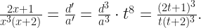
$\frac{2x + 1}{x^3(x + 2)} = \frac{d'}{a'} = \frac{d^3}{a^3} \cdot t^8 = \frac{(2t + 1)^3}{t(t + 2)^3}.$

Now we are almost done! Let us rewrite this a bit to show the polynomial we want to find roots of:

$\psi_{3, E_{a',d'}}(x) = x^3(x + 2)(2t + 1)^3 - (2x + 1)t(t + 2)^3.$

We know that we need to add some cubic root of some term in $k(t)$ in order to find the correct root. Exercise: use the results in the proof of Theorem 7 in Onuki and Montiya’s work, to show that we need the cubic root of $4t(t+1)$ . If Tate pairings are new to you, you can skip this exercise and use the result as a black box.

Adding this root $\alpha$ , our division polynomial will factor and give us the correct root! That means we can describe a point of order 3 on our curve $E_{a', d'}$ in terms of $t, \alpha$ .

This gives us all the material we need to compute the radical isogeny of degree 3 on a twisted² Edwards curve. Let’s move to section 3, fire up Sage/Magma, and compute!

3. Deriving formulas using Magma

In this section we finally derive the radical isogeny formula. This can probably be done by hand, but let’s use a computer algebra system to make things easier. I will use Magma to show how to compute the result described above, but you can do this in any reasonable computer algebra system. If you want to work along, you can always use the online Magma calculator here.

First, let us set-up the correct setting. We will factor the division polynomial over $k = \mathbb{Q}(t)$ , then the resulting formula will work for finite fields too.

Qt<t> := FunctionField(Rationals());
P<x> := PolynomialRing(Qt);

Luckily, we will not have to do too much with elliptic curves themselves, the twisted² Edwards form is not easy to do arithmetic with in Magma.

We define our 3-division polynomial we calculated above, and look at its factorization

psi3 := (2*x + 1)*t*(t+2)^3 - x^3*(x+2)*(2*t + 1)^3;

Factorization(psi3);
>
[
    <x + (1/2*t + 1)/(t + 1/2), 1>,
    <x^3 + 3/2*t/(t + 1/2)*x^2 + (-3/4*t^2 - 3/2*t)/(t^2 + t + 1/4)*x +
        (-1/4*t^3 - t^2 - t)/(t^2 + t + 1/4), 1>
]

We already find a root, without adding some cubic root?! Yes, we find the root associated to the dual isogeny of our initial Vélu isogeny. This is actually rather useless, as we would only end up at our original curve $E_{a,d}$ if we use this point. Hence, we need to add the cubic root $\alpha = \sqrt[3]{4t(t+1)}$ described above to factor the latter polynomial. We then redefine $\psi_3$ over the new field $\mathbb{Q}(t, \alpha)$ .

P<x> := PolynomialRing(Qta);
psi3 := P!psi3;
Factorization(psi3);
> 
[
    <x + (1/2*t + 1)/(t + 1/2), 1>,
    <x - 1/4/(t + 1/2)*a^2 - 1/2/(t + 1/2)*a + 1/2*t/(t + 1/2), 1>,
    <x^2 + (1/4/(t + 1/2)*a^2 + 1/2/(t + 1/2)*a + t/(t + 1/2))*x + (1/8*t +
        1/4)/(t^2 + t + 1/4)*a^2 + (1/4*t^2 + 1/2*t)/(t^2 + t + 1/4)*a +
        (-1/4*t^2 - 1/2*t)/(t^2 + t + 1/4), 1>
]

And there we find it! The root $\gamma$ that describes our radical isogeny of degree 3. Magma blurts it out in not the nicest form, but (exercise) we can rewrite $\gamma$ to get

$\gamma = \frac{\alpha^2 + 2(\alpha - t)}{2(2t +1)}.$

Curiously, this radical isogeny formula for twisted² Edwards curves is quite nice. It requires only one squaring and one multiplication, next to the exponentiation and the inversion. Especially when moving to projective coordinates (which makes sense when you’d want to integrate this into CSIDH) this formula is even cleaner than the ones on Montgomery curves and Tate normal curves. Of course, on Tate normal curves there exist radical isogeny formulas for degree 9, making the degree 3 formula rather obsolete. For more details on the projective coordinates and the challenges of integrating radical isogenies, see work by Chi-Domínguez and me (ePrint).

And that’s all: We’ve derived the radical isogeny formula for degree 3 on twisted² Edwards curves, using only a few ingredients. With this approach we’d be able to derive similar formulas for other curve forms for whatever form we prefer working on. For those up for a challenge, the next section describes how you’d find the degree 4 formula. For those who want to read more, check the last section to find further reading material!

Bonus: degree 4

As a bonus to the reader, we describe an extended exercise to compute the radical isogeny formula of degree 4 on twisted² Edwards curves.

First, look carefully at how Onuki and Moriya derive the radical isogeny formula for degree 4 on Montgomery curves.

Then, use the work by Moody and Shumow (see above) to figure out how 2-isogenies work on twisted² Edwards curves.

Finally, combine these approaches to compute a radical isogeny of degree 4 on twisted² Edwards curves, taking into account that for one needs to perform such isogenies on the surface of the isogeny graph (for more information on isogeny graphs for 2-isogenies, see the CSURF paper here by Castryck and Decru).

Reading material

I’ve linked a lot of reading material in this note, and I feel half-obliged to give some more details on why you might want to read these papers. I’ve also added some other papers that might be of interest. In order of appearence:

Radical isogenies. (by Castryck, Decru and Vercauteren, ePrint)
This paper originally introduces the ideas behind radical isogenies, and does a tremendous job at explaining much of the material that is not described in this note. The theoretical section describes most of the results we used here, and they derive explicit formulas for degrees 3 to 9.

Radical Isogenies on Montgomery Curves. (by Onuki and Moriya, ePrint)
This paper replicates the idea of radical isogenies to Montgomery curves, but also describes the connection of radical isogenies to modular curves. This really helps in understanding much more how radical isogenies fit into the bigger picture of elliptic curves. They derive their formulas for degree 3 and 4, and use the connection to modular curves to explain why degree 5 and higher is complicated on Montgomery curves.

On Kummer Lines With Full Rational 2-torsion and Their Usage in Cryptography. (by Hisil and Renes, PDF)
This paper describes in detail how Montgomery curves and twisted Edwards curves are connected, and furthermore describes how the Kummer line is very useful in isogeny-based cryptography. I have implicitly used these connections, but without explicitly mentioning this.

Two kinds of division polynomials for twisted Edwards curves. (by Moloney and McGuire, SpringerLink)
When you want to do radical isogenies on some curve form, you need division polynomials. Working those out by yourself is not the most fun. Luckily for us, Moloney and McGuire have done the work for us for twisted Edwards curves. A recommended read if you want to understand division polynomials in more detail.

Analogues of Vélu’s Formulas for Isogenies on Alternate Models of Elliptic Curves. (by Moody and Shumow, ePrint)
This paper’s title really says it all. They describe the analogues of Vélu’s formulas on alternate curve models, such as Edwards curves and Huff curves. The material is easily digestible and very readable, and should allow an interested reader to perform similar calculations for Huff curves.

Fully projective radical isogenies in constant-time. (by Chi-Domínguez and me, ePrint)
In this work we analyze how radical isogenies would perform in constant-time and provide projective formulas to increase their performance. Furthermore, we introduce a new (hybrid) strategy to improve the integration of radical isogenies into CSIDH. Unfortunately, we also find that radical isogenies give a lot of difficulties and do not really improve performance for CSIDH in large parameter sets.

CSIDH on the surface. (by Castryck and Decru, ePrint)
This paper introduced 2-isogenies to CSIDH, but perhaps the explanation on isogeny graphs is even more useful than 2-isogenies. Reading this paper in detail can greatly improve your understanding of CSIDH, isogeny graphs and particular choices of prime shapes that are useful in isogeny-based cryptography.

Additional reading

The Arithmetic of Elliptic Curves. (by Silverman, book)
The standard work to understand elliptic curves, isogenies, division polynomials, modular polynomials, pairings, … You name it, and it’s in here. For anyone in isogeny-based cryptography, Chapter III has at some point been required reading (and for good reason).

Twisted Edwards Curves. (by Bernstein, Birkner, Joye, Lange and Peters, ePrint)
The paper that originally introduced twisted Edwards curves as a generalization of Edwards curves. It explains why you would want to use twisted Edwards curves; they have some very nice properties when you want to do fast arithmetic!

1. Let’s get radical!

2. Towards twisted Edwards curves

3. Deriving formulas using Magma

Bonus: degree 4

Reading material

Share this:

Like this:

Leave a Reply Cancel reply